Last Time...

I focused on confounding and selection bias as two concepts in the causal inference(CI) literature that present serious obstacles to the project of good science. These were illustrated abstractly using directed acyclic graphs (DAGs) and concretely in the context of an example that looked at how ice cream flavor could potentially affect customers' experience at an ice cream store. In this post we'll depart from our ice cream example to bring things a little closer to my current area of research - examining how features of our built environment can potentially affect human health. We'll do this by looking at one of the most popular methods in CI: Instrumental Variables (IVs).

Instrumental Variables

As stated previously, IVs are one of the most popular tools in the CI literature. This is for good reason - while the investigation of causal effects outside the happy confines of a randomized clinical trial generally requires constant concerns over confounding and adjustment, IVs offer a path to causal inference outside these assumptions. However, nothing in life comes easy and IVs come with their own unique set of assumptions, the first set of which are appropriately named "the three instrumental conditions". Before we explore these and more in greater detail, let's return to a generic set-up in which we're interested in identifying some causal relationship.

In the figure below, variable $Y$ is the causal outcome of $X$ and $U$. $X$ is also causally determined by variable $Z$ which is independent of any of the other variables. If we're interested in identifying the causal effect of $X$ on $Y$ then we need to find some way to control for $U$ to ensure exchangeability. However, if we're unable to measure $U$, then there is still hope for us via the use of IVs!

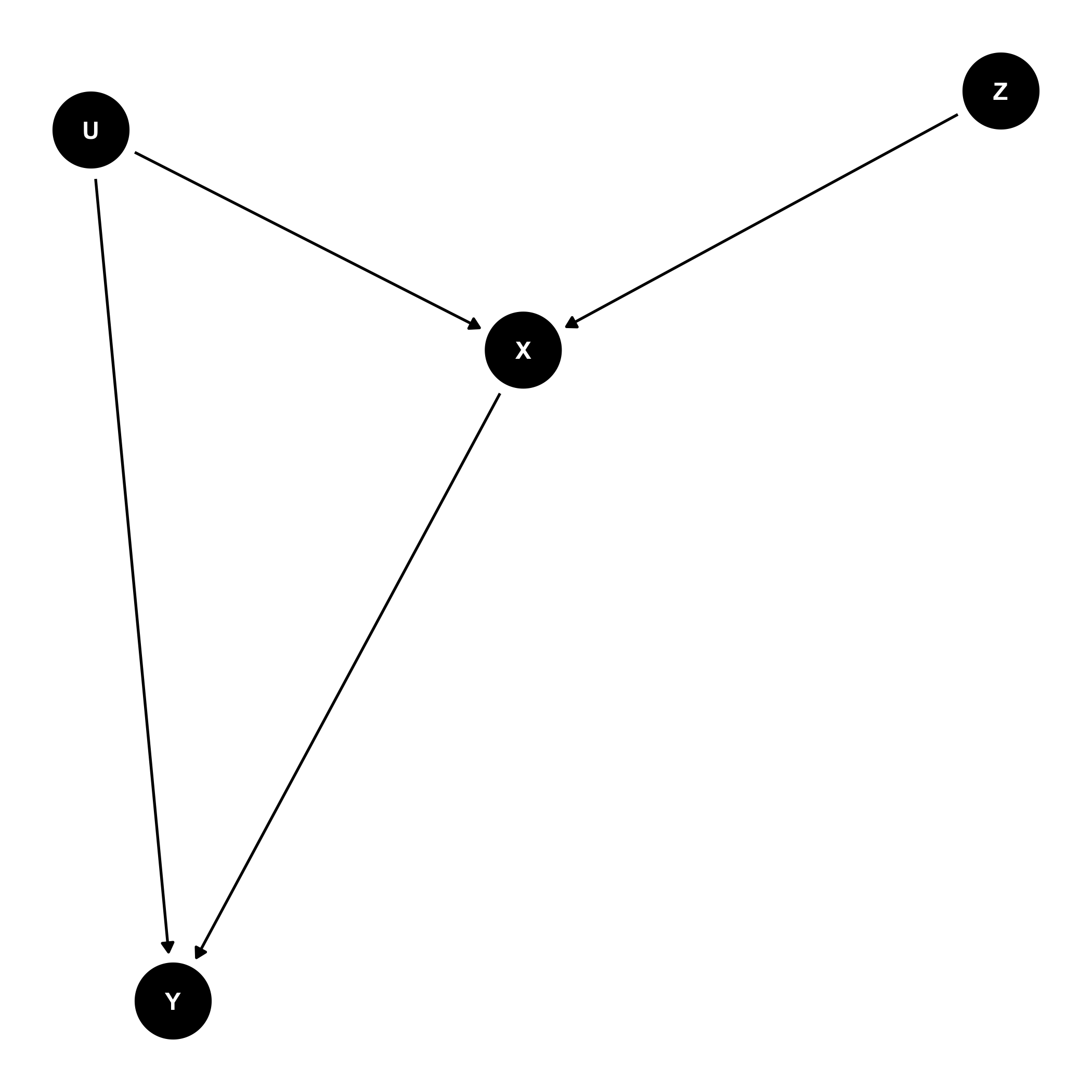
In our above example $Z$ could be used as an IV if it satisfies the three instrumental conditions, which are as follows:

1. $Z$ is associated with $X$.
2. $Z$ is not associated with $Y$ except through $X$.
3. $Z$ and $Y$ do not share causes.

The IV can be thought of as (amongst other things) a kind of upstream or proxy variable that measures what we're really interested in but are worried about confounding. For example, define $Z$ as the distance between individuals living in a city and the nearest fast food restaurant (FFR) to them. Similarly, define $X$ as excess junk food consumption, $Y$ as body mass index (BMI) and $U$ a (hypothetical) genetic factor that is linked to both excess junk food consumption as well as excess fat storage. In this case our diagram could be relabeled and we can now consider whether FFR distance satisfies the instrumental conditions.

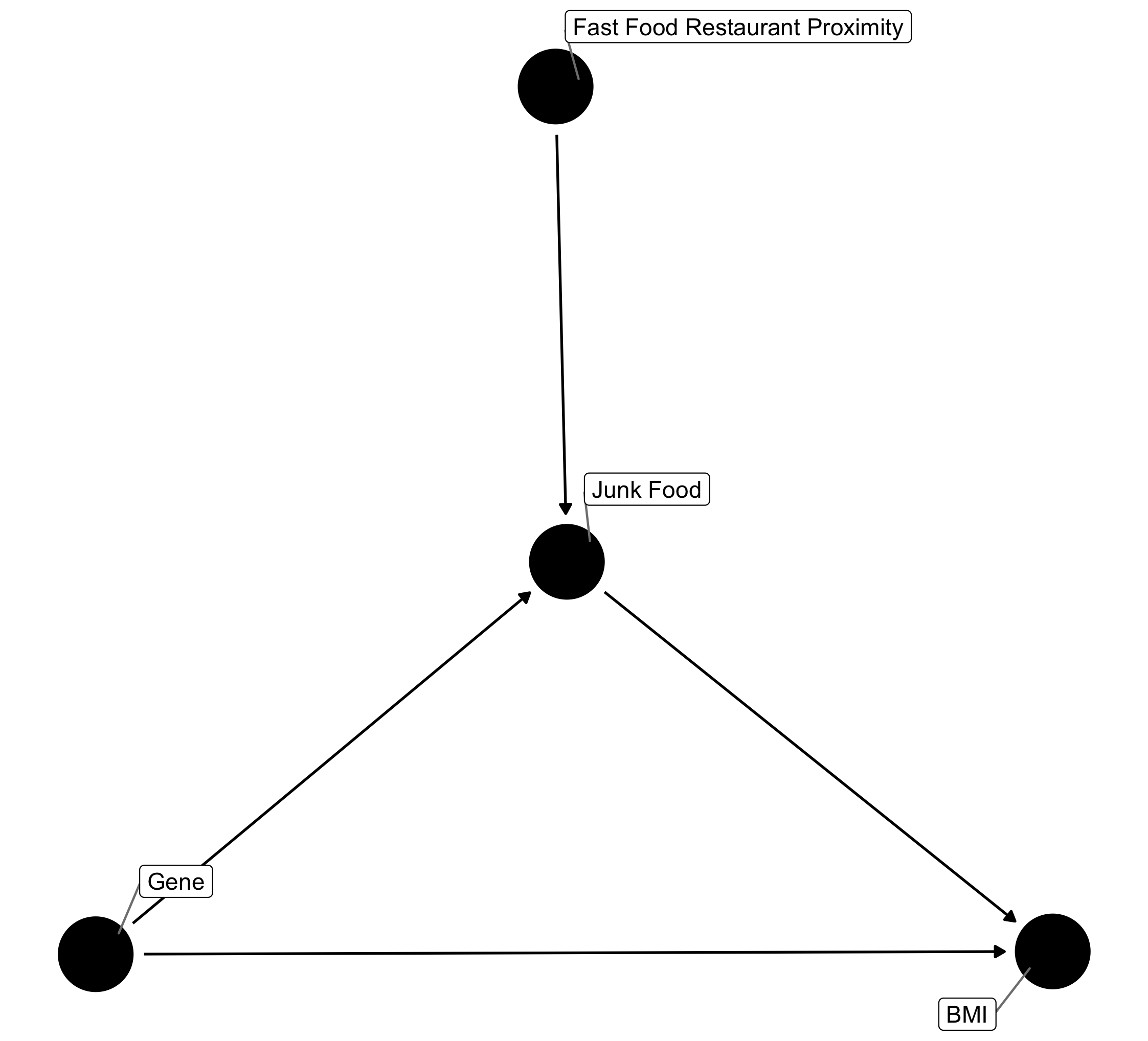
So does it satisfy the conditions? In order to determine this we need to ask the following questions, adapting the above to our specific case involving FFRs.

1. Is FFR proximity associated with excess junk food consumption?
2. Is FFR proximity independent of BMI except through excess junk food consumption?
3. Does FFR proximity share causes with BMI?

This is where things become tricky and why this example represents a departure from hypothetical to realistic. Let's work through these questions one-by-one in order to see how FFR proximity fails or succeeds to be an effective IV.

1. Is FFR proximity associated with excess junk food consumption?

Yes, though we may have to take this as a given in our case, if we had a specific dataset on hand we could test this for ourselves.

2. Is FFR proximity independent of BMI except through excess junk food consumption?

Certainly seems so, though as Hernan and Robbins point out, both this and the next assumption can never be truly verified. However, it is hard to imagine how being close to a modern FFR could increase/decrease one's BMI except through the consumption of fast food¹.

3. Does FFR proximity share causes with BMI?

Seems likely. After all, many FFRs are more likely to be in commercially-rich areas that typically also have a higher proportion of wealthy individuals. Since affluence is also a well known cause of BMI (determining one's ability to purchase healthy food or a gym membership for example), a backdoor path is created resulting in a new understanding of this causal framework.

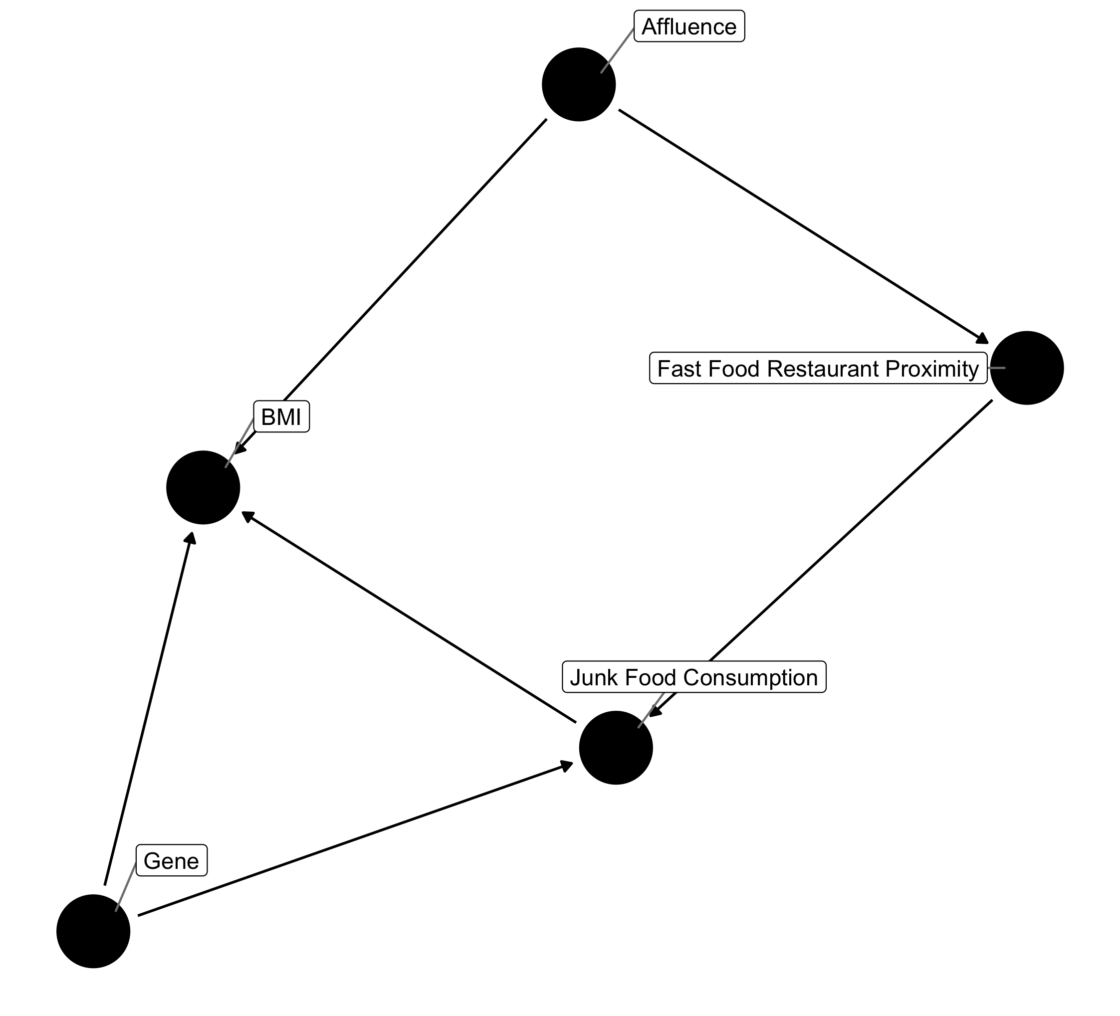
In order to remove this confounding and restore the ability of FFR proximity to act as an IV, we'll need to condition on subjects' income, or something similar, in order to account for the association between affluence and BMI².

With this obstacle overcome, are we done? Can we safely measure and use the distance between subjects and FFRs as an IV? Well ... not quite.

More Assumptions - Homogeneiety and Additivity

In our example, we're probably looking at more than one FFR and more than one type. McDonalds, Burger King, etc. are all commonly referred to as FFRs. If we're to lump these all together, do we assume they all have the same effect? This question speaks to the assumption of homogeneity and can be understood in relation to the consistency condition described in the preface blog post. If we're trying to estimate the causal effect of excess junk food consumption on BMI, it is not likely that all FFRs result in the same level of excess junk food consumption, however this may be an assumption we have to make. Furthermore, if we are to model the affect of multiple FFRs we will have to make some assumption as to whether the relationship is additive - linear in the number of FFRs - or nonlinear. Models that I've developed, that have been implemented in software like rstap and bbnet, make this assumption for computational and interpretable convenience, but it is likely not true³. As with most things in science, these assumptions are starting points upon which to build more sophisticated models that offer more flexibility.

Using FFR proximity as an IV

After all that work and assuming, we can finally use FFR proximity as an instrumental variable. The IV estimand for a binary IV would be:

\[ \hat{IV} = \frac{E[Y|Z=1]-E[Y|Z=0]}{E[A|Z=1]-E[A|Z=0]}. \]

By taking the ratio, the IV estimand tries to adjust the estimate of the change in $Y$ as a function of $Z$ by how strongly $Z$ predicts $A$. For a continuous variable, the estimand becomes:

\[ \hat{IV} = \frac{\text{Cov}(X,Y)}{\text{Cov}(A,Z)} = \frac{\text{Cov}(\text{FFR Proximity},BMI)}{\text{Cov}(\text{Calories of Junk Food},\text{FFR proximity})} . \]

This expression reflects the same idea.

In practice

In my work we rarely have data on junk food consumption, though some of the studies I've linked above did. Consequently, we're forced to look at the effect of $Z$ or FFR proximity on BMI without adjusting for the calories of junk food consumed, and hope that our data reflect the same relationships that have been shown in previous studies. It isn't neccessarily a bad assumption but certainly one that's worth being aware of and checking when possible.

Recap

In this blog post we learned about IV's and how they can be used to improve our ability to estimate what would otherwise be hard to measure causal effects. We worked through a specific example in which we considered access or proximity to FFRs as an instrumental variable and whether or not this measure would suffice as an IV under the IV conditions as well as what assumptions we would have to make in regards to homogeneiety and additivity. In the next blog post we'll complicate matters further, by considering what role time and time-varying confounders play in this causal framework.

Technical Notes

I produced the plots in this post using the ggdag R package, which extends the daggity R package.