A Recap and DAG intro
In the previous post I talked through some of the fundamental assumptions needed for Causal Inference as presented in Hernan and Robbins' textbook: (1) Exchangeability, (2) Positivity and (3) Consistency. In this post I'm planning to work through a brief discussion of two of the main obstacles to the fulfillment of the Exchangeability assumption: (1) Confounding and (2) Selection Bias. To do so, I'll be using Directed Acyclic Graphs or DAGS, which graphically represent the flow of causal information. If we were to consider our toy example from the preface post, on whether chocolate or vanilla ice cream results in a better ice cream store experience, the DAG that displays a causal relationship between these two variables would be the following:
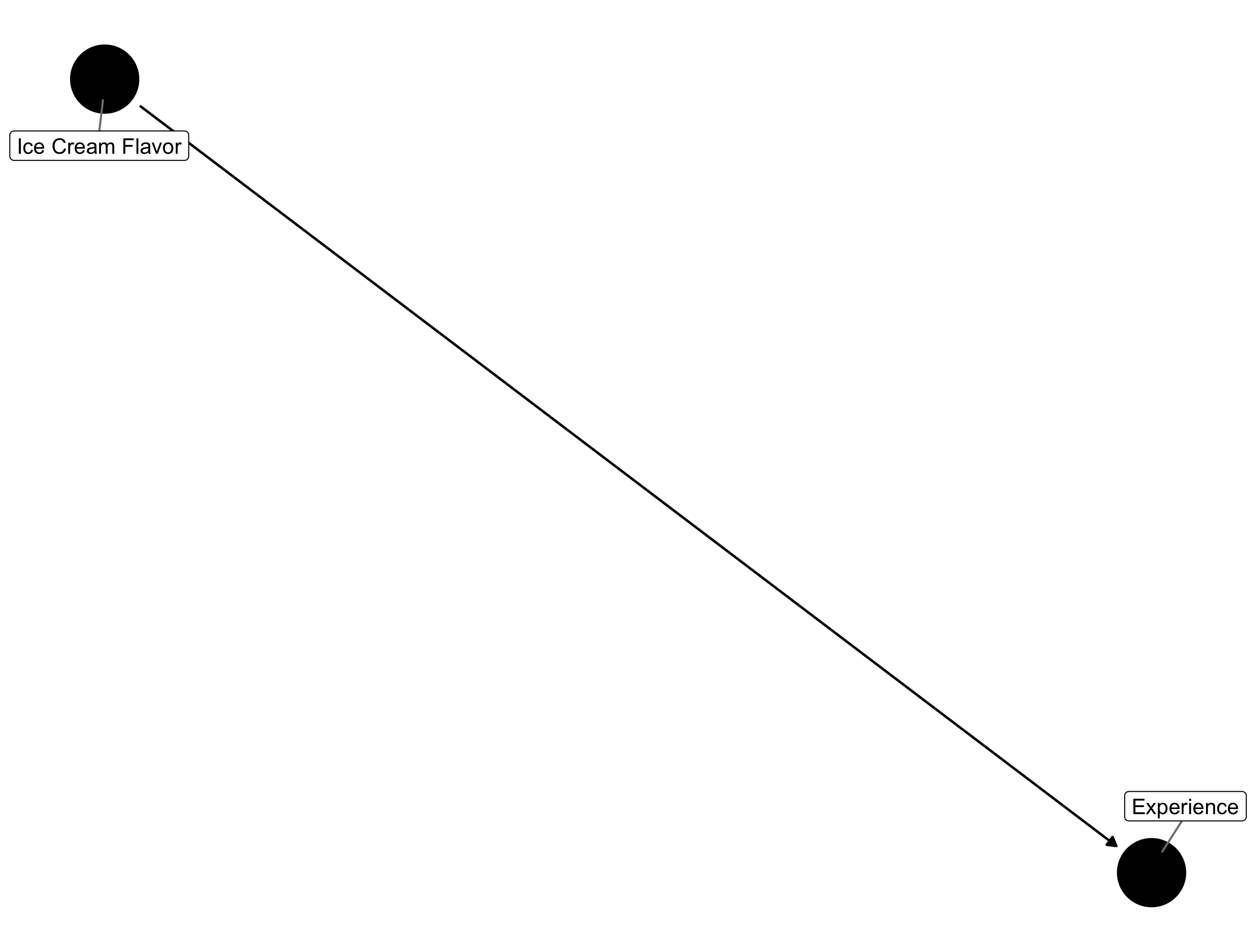
Ice Cream DAG
The arrow pointing from the ice cream flavor node towards the experience node indicates that we are positing a causal relationship between ice cream flavor and one's experience (on average). Simple, right? As we get into confounding and Selection Bias, we'll see how these plots can become more complicated.
Confounding: The Backdoor Path
The essential idea behind confounding is that there is some variable (a confounder) that is associated with both the causal intervention and outcome variable of interest. In terms of the causal DAG, it can be said that there is a "backdoor path" between the intervention and outcome variable of interest, through the confounder. Our ice cream example doesn't lend itself well to demonstrate this but suppose that people in a bad mood are more likely to order chocolate ice cream and, obviously, less likely to have a positive experience at the ice cream store. In this case, we would say that an individual's "background mood", confounds the effect of ice cream flavor on ice cream store experience and represent this idea using the following causal DAG.
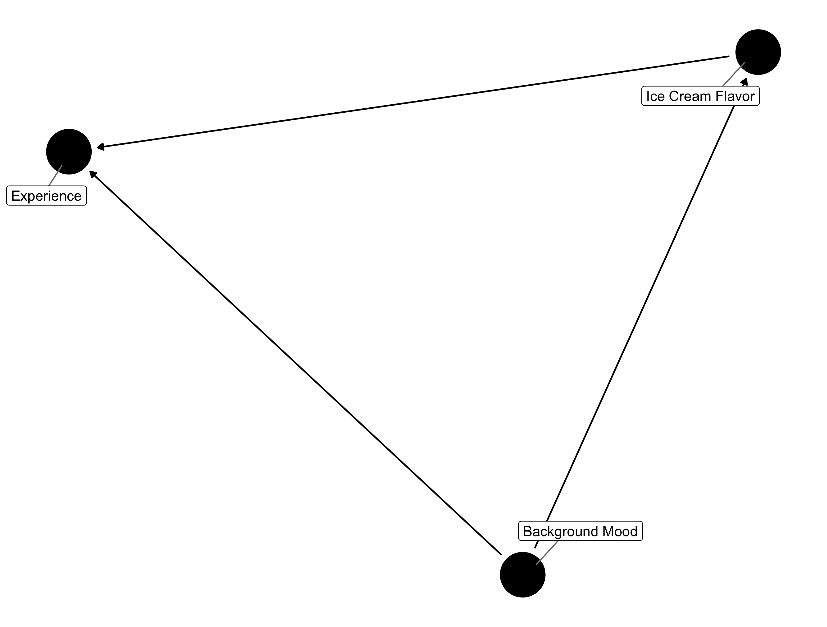
Confounding Ice Cream DAG
In order to address confounding we need to condition on some measure of an individual's background mood or some upstream variable that causally determines background mood. Suppose
the store worker marks on a sheet of paper their impression of whether a customer is in a bad mood or not. The causal effect of ice cream choice could now be
determined by looking at the probability of a positive ice cream store experience amongst those who had a bad experience and those who didn't and averaging over the probability
of being in a bad mood (this is a method called standardization), or alternatively, by including the bad mood indicator variable in a model like logistic regression. The DAG that
accounts for this adjustment looks like the following - note the changed color and shape in addition to the lighter shaded arrows.

Confounding Ice Cream DAG
In this example, conditioning on background mood ensures we have conditional exchangeability. If we failed to include or adjust for this information, our estimate of the causal effect of ice cream flavor would become biased, or incorrect. In more complicated examples, since we don't always know all the variables that could possibly confound the causal effect of interest, a scientist has to "assume conditional exchangeability" (as mentioned briefly in the preface), without ever knowing if this assumption is fully met.
There's more to be said here, as confounding often rears its' head in surprising ways. However, we'll stop here, leaving further examples for the textbook and turn our attention now to selection bias.
Selection Bias: The Unseen Filter
Selection bias refers to the bias or inaccuracy introduced to a causal effect estimate as a consequence for how the sample population is chosen or selected. In our ice cream store example, suppose that our chocolate ice cream is really bad. So bad in fact that that it makes costumer's less likely to fill out the post-purchase survey. Our results would become biased by this selection process and consequently, affect our estimate of ice cream choice on ice cream store experience. The updated causal DAG that would incorporate this information would look like the following, with an arrow pointing from the ice cream flavor to both the experience, and the censoring - whether or not we observed the data - variable.
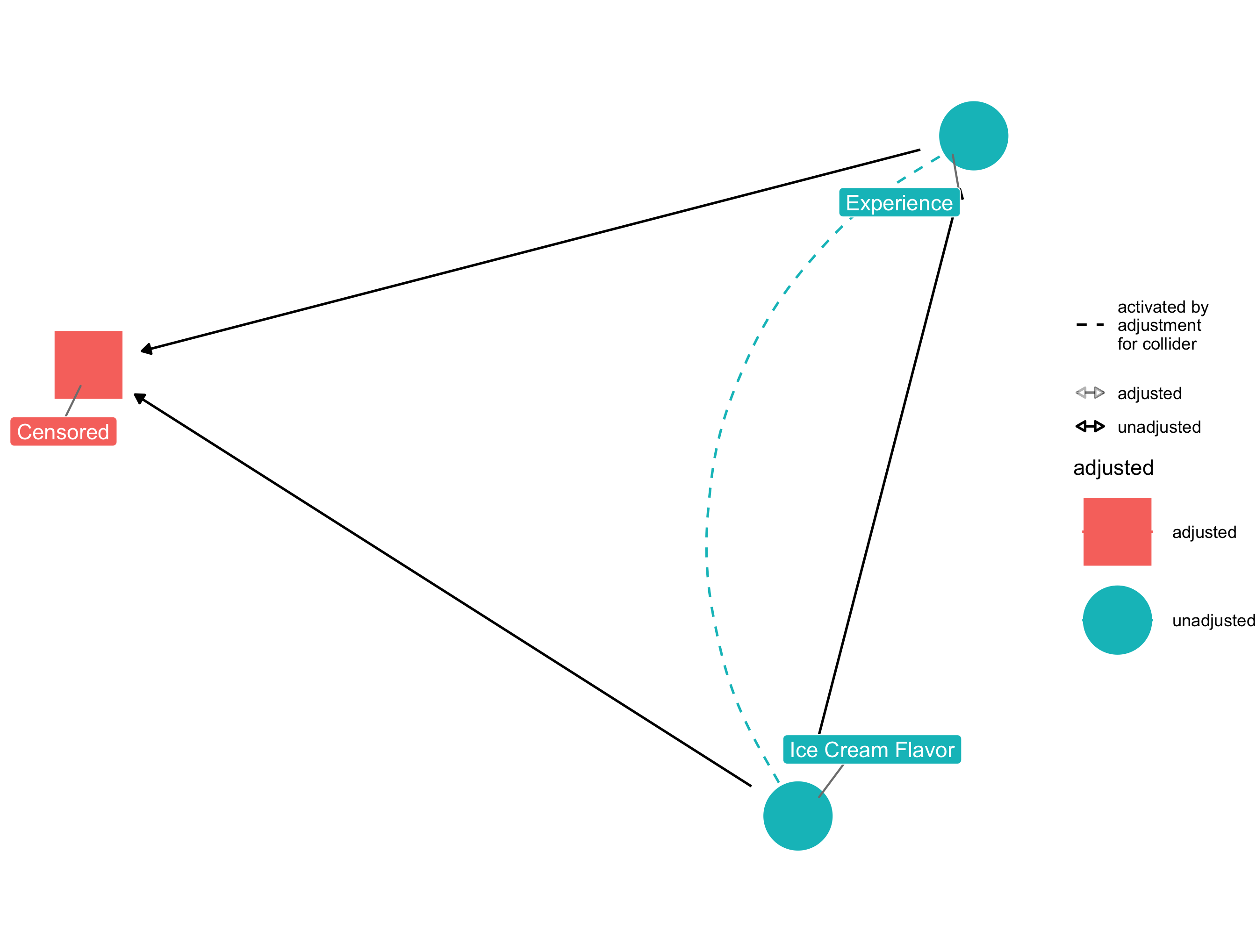
Selection Bias Ice Cream DAG
In causal DAG terms we would say that the censored variable is a collider, since it is causally determined by two variables. In order to adjust for this we'd need to incorporate the probability of censorship into our estimate of the effect of ice cream choice on ice cream store experience. This could be done through standardization (empirically integrating over the probability of censorship), IP weighting (same idea as standardization, formulated differently), or possibly stratification. The main idea behind both of these being that we need to take into account how likely someone is to be censored and/or restrict our analysis and inference to only those we observe. These methods will still rely on our assumptions of exchangeability, positivity and consistency, so in a real world analysis they will need to be re-checked in our causal diagram to ensure there isn't another confounder or other obstacle preventing identifiability.
As with confounding, there are a lot more details that can be found when examining selection bias, and I'd encourage the interested reader to check out chapter 8 of the aforementioned textbook, where Hernan and Robbins go through a number of different examples to jog readers' intuition on how to identify and address selection bias.
Onwards - to the Built Environment
Issues of both selection bias and confounding occur when examining the casual effect of features of the built environment. In fact, it can be extremely difficult to measure and detect just how where we live affects our health, because there are various mechanisms by which the effect may occur. In the next post I'll walk through the conditions for an instrumental variable and highlight how distance (or travel time) from a built environment feature (like a park or fast food restaurant) can be used as an instrumental variable, and examine what role confounding and selection bias play.
Technical Notes
I produced the plots in this post using the ggdag R package, which extends the daggity R package.